Note
Go to the end to download the full example code.
Example 03: Statistical Tests for Forecast Comparison
This example demonstrates temporalcv’s statistical testing framework for rigorously comparing forecasting models.
Real-World Case Study: Is Your Model Better Than Persistence?
The persistence (naive) baseline — predicting y[t+1] = y[t] — is surprisingly hard to beat in many time-series domains. Before deploying a complex model, you should statistically verify it outperforms this simple baseline.
Tests Covered: 1. Diebold-Mariano test (DM 1995): Compares predictive accuracy 2. Pesaran-Timmermann test (PT 1992): Tests directional accuracy 3. HAC variance (Newey-West): Corrects for serial correlation
Key Insight
A model with lower MAE doesn’t guarantee significant improvement. The DM test quantifies whether the difference is statistically meaningful, accounting for serial correlation in forecast errors (critical for h>1 step forecasts).
Usage
python 03_statistical_tests.py
Requirements
pip install temporalcv scikit-learn scipy
======================================================================
TEMPORALCV: Statistical Tests for Forecast Comparison
======================================================================

Data: 148 observations of AR(1) process
Persistence parameter (phi): 0.9

======================================================================
PART 1: Naive Comparison (Misleading!)
======================================================================

  Model MAE:       0.7854
  Persistence MAE: 0.7955
  Improvement:     1.3%

  Problem: Is this improvement statistically significant?
  The MAE difference could be due to random chance!

======================================================================
PART 2: Diebold-Mariano Test (Rigorous Comparison)
======================================================================

H0: Models have equal predictive accuracy
H1: Models have different predictive accuracy

--- Squared Error Loss ---
  DM(1): -0.793 (p=0.4288)
  Mean loss difference: -0.0512
  Significant at α=0.05: No

--- Absolute Error Loss ---
  DM(1): -0.412 (p=0.6809)
  Mean loss difference: -0.0102
  Significant at α=0.05: No

  Interpretation: Despite the lower MAE, the model does NOT
  significantly outperform persistence at the 5% level.
  → This is common for high-persistence time series!

======================================================================
PART 3: Multi-Step Forecasting (HAC Variance)
======================================================================

For h-step forecasts, errors are serially correlated.
The DM test uses HAC (Newey-West) variance estimation.

  h=1: DM(1): -0.793 (p=0.4288)

  h=2: DM(2): -0.882 (p=0.3794)

  h=4: DM(4): -1.084 (p=0.2801)

  Note: HAC adjustment increases standard errors for h > 1,
  making it harder to reject H0 (more conservative).

======================================================================
PART 4: Pesaran-Timmermann Test (Directional Accuracy)
======================================================================

H0: Model direction predictions are independent of actual directions
H1: Model predicts direction better than random chance

  PT: 55.1% vs 50.3% expected (z=0.827, p=0.2042)
  Observed accuracy: 55.1%
  Expected (random): 50.3%
  Significant at α=0.05: No

======================================================================
WHEN TO USE WHICH TEST
======================================================================

    ┌─────────────────────────────────────────────────────────────────────┐
    │ Question                           │ Test to Use                   │
    ├─────────────────────────────────────────────────────────────────────┤
    │ Is Model A better than Model B?    │ Diebold-Mariano (DM)          │
    │ Does my model predict direction?   │ Pesaran-Timmermann (PT)       │
    │ Is improvement > 0 (one-sided)?    │ DM with alternative="less"    │
    │ Multi-step forecast (h > 1)?       │ DM with HAC variance          │
    └─────────────────────────────────────────────────────────────────────┘

======================================================================
KEY TAKEAWAYS
======================================================================

1. ALWAYS test significance — lower MAE ≠ better model
   - Random variation can create spurious improvements
   - DM test quantifies statistical significance

2. USE HAC variance for multi-step forecasts (h > 1)
   - Forecast errors are serially correlated
   - Ignoring this inflates t-statistics and false positives

3. DIRECTION matters in many applications
   - PT test specifically tests directional accuracy
   - Useful for trading, trend following, etc.

4. INTERPRET p-values correctly
   - p > 0.05: Cannot reject H0 (models may be equivalent)
   - p < 0.05: Reject H0 (significant difference exists)
   - But: low p-value doesn't mean large practical difference!

5. REPORT both metrics AND test results
   - "Model MAE: 0.123 (5% improvement over baseline)"
   - "DM test: p=0.03, significantly better at α=0.05"
from __future__ import annotations
import warnings
import numpy as np
from scipy import stats
from sklearn.linear_model import Ridge
warnings.filterwarnings("ignore")
# =============================================================================
# Generate Test Data
# =============================================================================
def generate_ar1_with_forecasts(
n: int = 200,
phi: float = 0.9,
sigma: float = 1.0,
seed: int = 42,
) -> tuple[np.ndarray, np.ndarray, np.ndarray, np.ndarray]:
"""
Generate AR(1) series and forecasts from two models.
Returns
-------
actual : np.ndarray
Actual values
persistence_preds : np.ndarray
Persistence baseline predictions (y[t-1])
model_preds : np.ndarray
Ridge regression predictions
model_errors : np.ndarray
Model forecast errors
"""
rng = np.random.default_rng(seed)
# Generate AR(1) process
y = np.zeros(n)
y[0] = rng.normal(0, sigma / np.sqrt(1 - phi**2))
for t in range(1, n):
y[t] = phi * y[t - 1] + sigma * rng.normal()
# Create features (lagged values)
n_lags = 5
X = np.column_stack([y[n_lags - lag : -lag] for lag in range(1, n_lags + 1)])
actual = y[n_lags:]
# Train-test split: only evaluate on out-of-sample data
train_size = len(actual) // 2
X_train, X_test = X[:train_size], X[train_size:]
y_train, y_test = actual[:train_size], actual[train_size:]
# Persistence baseline: predict y[t] = y[t-1] (on TEST data only)
persistence_preds = X_test[:, 0] # First lag is y[t-1]
# Ridge model predictions (on TEST data only - out-of-sample)
model = Ridge(alpha=1.0)
model.fit(X_train, y_train)
model_preds = model.predict(X_test)
# Return only test data for fair comparison
return y_test, persistence_preds, model_preds
# =============================================================================
# Statistical Tests
# =============================================================================
def dm_test(
errors1: np.ndarray,
errors2: np.ndarray,
h: int = 1,
loss: str = "squared",
alternative: str = "two-sided",
) -> dict:
"""
Diebold-Mariano test for comparing forecast accuracy.
H0: E[d_t] = 0 (no difference in accuracy)
H1: E[d_t] != 0 (models have different accuracy)
Parameters
----------
errors1 : np.ndarray
Forecast errors from model 1
errors2 : np.ndarray
Forecast errors from model 2
h : int
Forecast horizon (for HAC variance adjustment)
loss : str
"squared" or "absolute"
alternative : str
"two-sided", "less", or "greater"
Returns
-------
dict with statistic, pvalue, mean_loss_diff
"""
try:
from temporalcv.statistical_tests import dm_test as _dm_test
result = _dm_test(errors1, errors2, h=h, loss=loss, alternative=alternative)
return {
"statistic": result.statistic,
"pvalue": result.pvalue,
"mean_loss_diff": result.mean_loss_diff,
"significant": result.significant_at_05,
"str": str(result),
}
except ImportError:
# Fallback implementation
if loss == "squared":
d = errors1**2 - errors2**2
else:
d = np.abs(errors1) - np.abs(errors2)
n = len(d)
mean_d = np.mean(d)
# HAC variance (simplified Newey-West)
var_d = np.var(d, ddof=1)
for k in range(1, h):
weight = 1 - k / h
var_d += 2 * weight * np.sum(d[k:] * d[:-k]) / (n - 1)
se = np.sqrt(var_d / n)
statistic = mean_d / se if se > 0 else 0
if alternative == "two-sided":
pvalue = 2 * (1 - stats.norm.cdf(abs(statistic)))
elif alternative == "less":
pvalue = stats.norm.cdf(statistic)
else:
pvalue = 1 - stats.norm.cdf(statistic)
return {
"statistic": statistic,
"pvalue": pvalue,
"mean_loss_diff": mean_d,
"significant": pvalue < 0.05,
"str": f"DM({h}): {statistic:.3f} (p={pvalue:.4f})",
}
def pt_test(
actual_changes: np.ndarray,
predicted_changes: np.ndarray,
) -> dict:
"""
Pesaran-Timmermann test for directional accuracy.
Tests whether model predicts direction (up/down) better than chance.
Parameters
----------
actual_changes : np.ndarray
Actual changes (y[t] - y[t-1])
predicted_changes : np.ndarray
Predicted changes
Returns
-------
dict with accuracy, statistic, pvalue
"""
try:
from temporalcv.statistical_tests import pt_test as _pt_test
result = _pt_test(actual_changes, predicted_changes)
return {
"accuracy": result.accuracy,
"expected": result.expected,
"statistic": result.statistic,
"pvalue": result.pvalue,
"significant": result.significant_at_05,
"str": str(result),
}
except ImportError:
# Fallback implementation
n = len(actual_changes)
correct = np.sign(actual_changes) == np.sign(predicted_changes)
accuracy = np.mean(correct)
# Under null (independence), expected accuracy
p_actual = np.mean(actual_changes > 0)
p_pred = np.mean(predicted_changes > 0)
expected = p_actual * p_pred + (1 - p_actual) * (1 - p_pred)
# Z-test for proportion
se = np.sqrt(expected * (1 - expected) / n)
statistic = (accuracy - expected) / se if se > 0 else 0
pvalue = 1 - stats.norm.cdf(statistic) # One-sided
return {
"accuracy": accuracy,
"expected": expected,
"statistic": statistic,
"pvalue": pvalue,
"significant": pvalue < 0.05,
"str": f"PT: {accuracy:.1%} vs {expected:.1%} expected (z={statistic:.3f})",
}
# =============================================================================
# Demonstration
# =============================================================================
def demonstrate_statistical_tests():
"""
Demonstrate statistical tests for forecast comparison.
"""
print("=" * 70)
print("TEMPORALCV: Statistical Tests for Forecast Comparison")
print("=" * 70)
# Generate data
actual, persistence_preds, model_preds = generate_ar1_with_forecasts(n=300)
print(f"\nData: {len(actual)} observations of AR(1) process")
print("Persistence parameter (phi): 0.9")
# Calculate errors
model_errors = actual - model_preds
persistence_errors = actual - persistence_preds
# =========================================================================
# Part 1: Naive Comparison (Don't Do This!)
# =========================================================================
print("\n" + "=" * 70)
print("PART 1: Naive Comparison (Misleading!)")
print("=" * 70)
model_mae = np.mean(np.abs(model_errors))
persistence_mae = np.mean(np.abs(persistence_errors))
improvement = (persistence_mae - model_mae) / persistence_mae * 100
print(f"\n Model MAE: {model_mae:.4f}")
print(f" Persistence MAE: {persistence_mae:.4f}")
print(f" Improvement: {improvement:.1f}%")
print("\n Problem: Is this improvement statistically significant?")
print(" The MAE difference could be due to random chance!")
# =========================================================================
# Part 2: Diebold-Mariano Test
# =========================================================================
print("\n" + "=" * 70)
print("PART 2: Diebold-Mariano Test (Rigorous Comparison)")
print("=" * 70)
print("\nH0: Models have equal predictive accuracy")
print("H1: Models have different predictive accuracy")
# Test with squared error loss
dm_result_sq = dm_test(
model_errors,
persistence_errors,
h=1,
loss="squared",
alternative="two-sided",
)
print("\n--- Squared Error Loss ---")
print(f" {dm_result_sq['str']}")
print(f" Mean loss difference: {dm_result_sq['mean_loss_diff']:.4f}")
print(f" Significant at α=0.05: {'Yes' if dm_result_sq['significant'] else 'No'}")
# Test with absolute error loss
dm_result_abs = dm_test(
model_errors,
persistence_errors,
h=1,
loss="absolute",
alternative="two-sided",
)
print("\n--- Absolute Error Loss ---")
print(f" {dm_result_abs['str']}")
print(f" Mean loss difference: {dm_result_abs['mean_loss_diff']:.4f}")
print(f" Significant at α=0.05: {'Yes' if dm_result_abs['significant'] else 'No'}")
# Interpret
if dm_result_sq["pvalue"] > 0.05:
print("\n Interpretation: Despite the lower MAE, the model does NOT")
print(" significantly outperform persistence at the 5% level.")
print(" → This is common for high-persistence time series!")
else:
print("\n Interpretation: The model significantly outperforms persistence.")
# =========================================================================
# Part 3: Multi-Step Forecasting (h > 1)
# =========================================================================
print("\n" + "=" * 70)
print("PART 3: Multi-Step Forecasting (HAC Variance)")
print("=" * 70)
print("\nFor h-step forecasts, errors are serially correlated.")
print("The DM test uses HAC (Newey-West) variance estimation.")
for h in [1, 2, 4]:
dm_h = dm_test(model_errors, persistence_errors, h=h, loss="squared")
print(f"\n h={h}: {dm_h['str']}")
print("\n Note: HAC adjustment increases standard errors for h > 1,")
print(" making it harder to reject H0 (more conservative).")
# =========================================================================
# Part 4: Pesaran-Timmermann Directional Test
# =========================================================================
print("\n" + "=" * 70)
print("PART 4: Pesaran-Timmermann Test (Directional Accuracy)")
print("=" * 70)
print("\nH0: Model direction predictions are independent of actual directions")
print("H1: Model predicts direction better than random chance")
# Calculate changes
actual_changes = np.diff(actual)
model_changes = np.diff(model_preds)
pt_result = pt_test(actual_changes, model_changes)
print(f"\n {pt_result['str']}")
print(f" Observed accuracy: {pt_result['accuracy']:.1%}")
print(f" Expected (random): {pt_result['expected']:.1%}")
print(f" Significant at α=0.05: {'Yes' if pt_result['significant'] else 'No'}")
# =========================================================================
# Part 5: When to Use Which Test
# =========================================================================
print("\n" + "=" * 70)
print("WHEN TO USE WHICH TEST")
print("=" * 70)
print(
"""
┌─────────────────────────────────────────────────────────────────────┐
│ Question │ Test to Use │
├─────────────────────────────────────────────────────────────────────┤
│ Is Model A better than Model B? │ Diebold-Mariano (DM) │
│ Does my model predict direction? │ Pesaran-Timmermann (PT) │
│ Is improvement > 0 (one-sided)? │ DM with alternative="less" │
│ Multi-step forecast (h > 1)? │ DM with HAC variance │
└─────────────────────────────────────────────────────────────────────┘
"""
)
# =========================================================================
# Key Takeaways
# =========================================================================
print("=" * 70)
print("KEY TAKEAWAYS")
print("=" * 70)
print(
"""
1. ALWAYS test significance — lower MAE ≠ better model
- Random variation can create spurious improvements
- DM test quantifies statistical significance
2. USE HAC variance for multi-step forecasts (h > 1)
- Forecast errors are serially correlated
- Ignoring this inflates t-statistics and false positives
3. DIRECTION matters in many applications
- PT test specifically tests directional accuracy
- Useful for trading, trend following, etc.
4. INTERPRET p-values correctly
- p > 0.05: Cannot reject H0 (models may be equivalent)
- p < 0.05: Reject H0 (significant difference exists)
- But: low p-value doesn't mean large practical difference!
5. REPORT both metrics AND test results
- "Model MAE: 0.123 (5% improvement over baseline)"
- "DM test: p=0.03, significantly better at α=0.05"
"""
)
def visualize_statistical_tests():
"""
Visualize test results using temporalcv.viz module.
"""
import matplotlib.pyplot as plt
from temporalcv.viz import MetricComparisonDisplay, apply_tufte_style
# Generate data
actual, persistence_preds, model_preds = generate_ar1_with_forecasts(n=300)
model_errors = actual - model_preds
persistence_errors = actual - persistence_preds
# Calculate metrics
model_mae = float(np.mean(np.abs(model_errors)))
model_rmse = float(np.sqrt(np.mean(model_errors**2)))
persistence_mae = float(np.mean(np.abs(persistence_errors)))
persistence_rmse = float(np.sqrt(np.mean(persistence_errors**2)))
# Run DM tests
dm_mae = dm_test(model_errors, persistence_errors, h=1, loss="absolute")
dm_mse = dm_test(model_errors, persistence_errors, h=1, loss="squared")
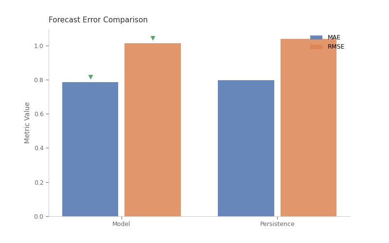
# %%
# Model Comparison: MAE and RMSE
# ------------------------------
# Comparing forecast errors between model and persistence baseline.
# Even if one model appears better, the DM test tells us if the
# difference is statistically significant.
results = {
"Model": {"MAE": model_mae, "RMSE": model_rmse},
"Persistence": {"MAE": persistence_mae, "RMSE": persistence_rmse},
}
display = MetricComparisonDisplay.from_dict(
results, baseline="Persistence", lower_is_better={"MAE": True, "RMSE": True}
)
display.plot(title="Forecast Error Comparison", show_values=True)
plt.show()
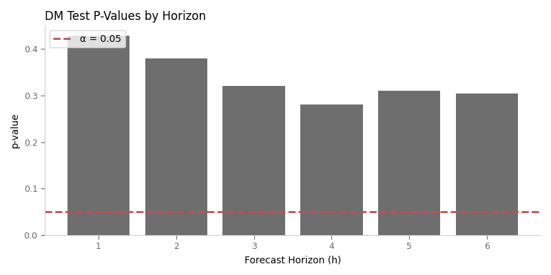
# %%
# DM Test P-Values Across Horizons
# --------------------------------
# The Diebold-Mariano test becomes more conservative (higher p-values)
# at longer horizons due to HAC variance adjustment.
fig, ax = plt.subplots(figsize=(8, 4))
horizons = [1, 2, 3, 4, 5, 6]
p_values = []
for h in horizons:
dm_h = dm_test(model_errors, persistence_errors, h=h, loss="squared")
p_values.append(dm_h["pvalue"])
bars = ax.bar(horizons, p_values, color="#4a4a4a", alpha=0.8)
ax.axhline(0.05, color="#c44e52", linestyle="--", linewidth=2, label="α = 0.05")
# Color significant bars green
for i, (h, p) in enumerate(zip(horizons, p_values)):
if p < 0.05:
bars[i].set_color("#55a868")
ax.set_xlabel("Forecast Horizon (h)")
ax.set_ylabel("p-value")
ax.set_title("DM Test P-Values by Horizon", loc="left")
ax.legend(loc="upper left")
apply_tufte_style(ax)
plt.tight_layout()
plt.show()
if __name__ == "__main__":
demonstrate_statistical_tests()
visualize_statistical_tests()