Example 04: Handling High-Persistence Time Series

This example demonstrates how to validate models on high-persistence data (ACF(1) > 0.9) where standard metrics can be misleading.

Real-World Case Study: Interest Rate Forecasting

Treasury rates, exchange rates, and many financial series have ACF(1) > 0.95. On such data: - Persistence (naive) baseline has near-zero error - Complex models struggle to beat persistence - Standard CV metrics overestimate performance

Key Metrics for High-Persistence Data: - MC-SS ratio: Model Change vs Seasonally-adjusted Series scale - MASE: Mean Absolute Scaled Error (relative to naive baseline) - DM test: Statistical comparison to persistence

Usage

python 04_high_persistence.py

Requirements

pip install temporalcv scikit-learn

from __future__ import annotations

import warnings

import matplotlib.pyplot as plt
import numpy as np
from sklearn.ensemble import GradientBoostingRegressor
from sklearn.linear_model import Ridge

from temporalcv.viz import apply_tufte_style

warnings.filterwarnings("ignore")


# =============================================================================
# Generate High-Persistence Data
# =============================================================================


def generate_high_persistence_data(
    n: int = 500,
    phi: float = 0.98,  # Very high persistence
    sigma: float = 0.05,
    seed: int = 42,
) -> np.ndarray:
    """Generate high-persistence AR(1) process (like Treasury rates)."""
    rng = np.random.default_rng(seed)
    y = np.zeros(n)
    y[0] = 3.0 + rng.normal(0, sigma / np.sqrt(1 - phi**2))

    for t in range(1, n):
        y[t] = phi * y[t - 1] + (1 - phi) * 3.0 + sigma * rng.normal()

    return y


def create_features(series: np.ndarray, n_lags: int = 5):
    """Create lagged features."""
    n = len(series)
    features = []
    for lag in range(1, n_lags + 1):
        lagged = np.full(n, np.nan)
        lagged[lag:] = series[:-lag]
        features.append(lagged)
    X = np.column_stack(features)
    y = series.copy()
    valid = ~np.isnan(X).any(axis=1)
    return X[valid], y[valid]


# =============================================================================
# Metrics for High-Persistence Data
# =============================================================================


def compute_mase(actual: np.ndarray, predicted: np.ndarray, train_data: np.ndarray = None) -> float:
    """
    Mean Absolute Scaled Error (Hyndman & Koehler 2006).

    MASE < 1: Better than naive baseline
    MASE = 1: Same as naive
    MASE > 1: Worse than naive

    Parameters
    ----------
    actual : np.ndarray
        Test set actual values
    predicted : np.ndarray
        Model predictions on test set
    train_data : np.ndarray, optional
        Training data for computing naive baseline scale.
        If None, uses actual (test data) for backward compatibility,
        but this is NOT recommended per MASE definition.
    """
    mae = np.mean(np.abs(actual - predicted))
    # Naive baseline MAE should be computed from TRAINING data per MASE definition
    if train_data is not None:
        naive_mae = np.mean(np.abs(np.diff(train_data)))
    else:
        # Fallback: compute from test data (not recommended)
        naive_mae = np.mean(np.abs(np.diff(actual)))
    return mae / naive_mae if naive_mae > 0 else np.inf


def compute_mc_ss_ratio(actual: np.ndarray, predicted: np.ndarray) -> float:
    """
    Model Change vs Series Scale ratio.

    For high-persistence data, changes are tiny relative to series level.
    This metric normalizes by the series scale.
    """
    mae = np.mean(np.abs(actual - predicted))
    series_scale = np.std(actual)
    return mae / series_scale if series_scale > 0 else np.inf


def compute_directional_accuracy(actual: np.ndarray, predicted: np.ndarray) -> float:
    """Proportion of correct direction predictions."""
    actual_changes = np.diff(actual)
    pred_changes = np.diff(predicted)
    return np.mean(np.sign(actual_changes) == np.sign(pred_changes))


# =============================================================================
# Demonstration
# =============================================================================


def demonstrate_high_persistence():
    """Demonstrate handling of high-persistence data."""
    print("=" * 70)
    print("TEMPORALCV: Handling High-Persistence Time Series")
    print("=" * 70)

    # Generate data
    series = generate_high_persistence_data()
    acf1 = np.corrcoef(series[1:], series[:-1])[0, 1]
    print("\nData characteristics:")
    print(f"  Length: {len(series)}")
    print(f"  Mean: {np.mean(series):.2f}")
    print(f"  Std: {np.std(series):.4f}")
    print(f"  ACF(1): {acf1:.4f} (HIGH persistence)")

    # Create features
    X, y = create_features(series)
    train_size = int(0.7 * len(y))

    X_train, X_test = X[:train_size], X[train_size:]
    y_train, y_test = y[:train_size], y[train_size:]

    print(f"\n  Train: {len(X_train)} samples")
    print(f"  Test: {len(X_test)} samples")

    # =========================================================================
    # Part 1: The Persistence Baseline Problem
    # =========================================================================
    print("\n" + "=" * 70)
    print("PART 1: The Persistence Baseline Problem")
    print("=" * 70)

    # Persistence predictions
    persistence_preds = X_test[:, 0]  # y[t-1]

    persistence_mae = np.mean(np.abs(y_test - persistence_preds))
    print(f"\n  Persistence baseline MAE: {persistence_mae:.6f}")
    print("  Persistence MASE: 1.000 (by definition)")
    print("  This is an EXTREMELY tough baseline to beat!")

    # =========================================================================
    # Part 2: Model Comparison
    # =========================================================================
    print("\n" + "=" * 70)
    print("PART 2: Model Comparison")
    print("=" * 70)

    models = {
        "Ridge (simple)": Ridge(alpha=1.0),
        "GBM (complex)": GradientBoostingRegressor(n_estimators=50, max_depth=2, random_state=42),
    }

    results = []
    for name, model in models.items():
        model.fit(X_train, y_train)
        preds = model.predict(X_test)

        mae = np.mean(np.abs(y_test - preds))
        # Pass y_train for MASE denominator per Hyndman & Koehler 2006
        mase = compute_mase(y_test, preds, train_data=y_train)
        mc_ss = compute_mc_ss_ratio(y_test, preds)
        dir_acc = compute_directional_accuracy(y_test, preds)

        results.append(
            {
                "name": name,
                "mae": mae,
                "mase": mase,
                "mc_ss": mc_ss,
                "dir_acc": dir_acc,
            }
        )

        print(f"\n  {name}:")
        print(f"    MAE:  {mae:.6f} (vs persistence: {persistence_mae:.6f})")
        print(f"    MASE: {mase:.3f} {'✓ <1' if mase < 1 else '✗ ≥1'}")
        print(f"    MC/SS: {mc_ss:.3f}")
        print(f"    Direction accuracy: {dir_acc:.1%}")

    # =========================================================================
    # Part 3: Why Standard Metrics Mislead
    # =========================================================================
    print("\n" + "=" * 70)
    print("PART 3: Why Standard Metrics Mislead")
    print("=" * 70)

    print(
        """
    For high-persistence data (ACF(1) > 0.95):

    ┌─────────────────────────────────────────────────────────────────────┐
    │ Metric   │ Problem                          │ Better Alternative    │
    ├─────────────────────────────────────────────────────────────────────┤
    │ MAE/RMSE │ Near-zero for persistence        │ MASE (scaled)         │
    │ R²       │ Near 1.0 even for naive models   │ Out-of-sample R²      │
    │ % Error  │ Meaningless when y ≈ constant    │ Relative to baseline  │
    └─────────────────────────────────────────────────────────────────────┘
    """
    )

    # =========================================================================
    # Part 4: Validation Strategy
    # =========================================================================
    print("=" * 70)
    print("PART 4: Recommended Validation Strategy")
    print("=" * 70)
    print(
        """
1. ALWAYS compare to persistence baseline
   - If MASE ≥ 1, your model doesn't beat naive
   - Use DM test to verify statistical significance

2. LOOK at directional accuracy
   - Even 55% accuracy can be valuable for trading
   - Use PT test for statistical significance

3. USE walk-forward CV with sufficient gap
   - Prevents leakage from feature engineering
   - Reflects realistic deployment scenario

4. MONITOR regime changes
   - High-persistence ≠ stationary
   - Sliding window may outperform expanding

5. BE SKEPTICAL of impressive metrics
   - MAE of 0.001 is meaningless if persistence achieves 0.0005
   - Always report relative metrics (MASE, % improvement)
"""
    )

    # =========================================================================
    # Part 5: Summary Table
    # =========================================================================
    print("=" * 70)
    print("SUMMARY TABLE")
    print("=" * 70)
    print(f"\n{'Model':<20} {'MAE':<12} {'MASE':<8} {'Direction':<10} {'Verdict':<15}")
    print("-" * 65)
    print(f"{'Persistence':<20} {persistence_mae:<12.6f} {'1.000':<8} {'-':<10} {'Baseline':<15}")
    for r in results:
        verdict = "✓ Better" if r["mase"] < 1 else "✗ No better"
        print(
            f"{r['name']:<20} {r['mae']:<12.6f} {r['mase']:<8.3f} {r['dir_acc']:<10.1%} {verdict:<15}"
        )


if __name__ == "__main__":
    demonstrate_high_persistence()

======================================================================
TEMPORALCV: Handling High-Persistence Time Series
======================================================================

Data characteristics:
  Length: 500
  Mean: 2.98
  Std: 0.1695
  ACF(1): 0.9593 (HIGH persistence)

  Train: 346 samples
  Test: 149 samples

======================================================================
PART 1: The Persistence Baseline Problem
======================================================================

  Persistence baseline MAE: 0.039061
  Persistence MASE: 1.000 (by definition)
  This is an EXTREMELY tough baseline to beat!

======================================================================
PART 2: Model Comparison
======================================================================

  Ridge (simple):
    MAE:  0.046039 (vs persistence: 0.039061)
    MASE: 1.222 ✗ ≥1
    MC/SS: 0.268
    Direction accuracy: 50.7%

  GBM (complex):
    MAE:  0.043450 (vs persistence: 0.039061)
    MASE: 1.154 ✗ ≥1
    MC/SS: 0.253
    Direction accuracy: 50.0%

======================================================================
PART 3: Why Standard Metrics Mislead
======================================================================

    For high-persistence data (ACF(1) > 0.95):

    ┌─────────────────────────────────────────────────────────────────────┐
    │ Metric   │ Problem                          │ Better Alternative    │
    ├─────────────────────────────────────────────────────────────────────┤
    │ MAE/RMSE │ Near-zero for persistence        │ MASE (scaled)         │
    │ R²       │ Near 1.0 even for naive models   │ Out-of-sample R²      │
    │ % Error  │ Meaningless when y ≈ constant    │ Relative to baseline  │
    └─────────────────────────────────────────────────────────────────────┘

======================================================================
PART 4: Recommended Validation Strategy
======================================================================

1. ALWAYS compare to persistence baseline
   - If MASE ≥ 1, your model doesn't beat naive
   - Use DM test to verify statistical significance

2. LOOK at directional accuracy
   - Even 55% accuracy can be valuable for trading
   - Use PT test for statistical significance

3. USE walk-forward CV with sufficient gap
   - Prevents leakage from feature engineering
   - Reflects realistic deployment scenario

4. MONITOR regime changes
   - High-persistence ≠ stationary
   - Sliding window may outperform expanding

5. BE SKEPTICAL of impressive metrics
   - MAE of 0.001 is meaningless if persistence achieves 0.0005
   - Always report relative metrics (MASE, % improvement)

======================================================================
SUMMARY TABLE
======================================================================

Model                MAE          MASE     Direction  Verdict
-----------------------------------------------------------------
Persistence          0.039061     1.000    -          Baseline
Ridge (simple)       0.046039     1.222    50.7%      ✗ No better
GBM (complex)        0.043450     1.154    50.0%      ✗ No better

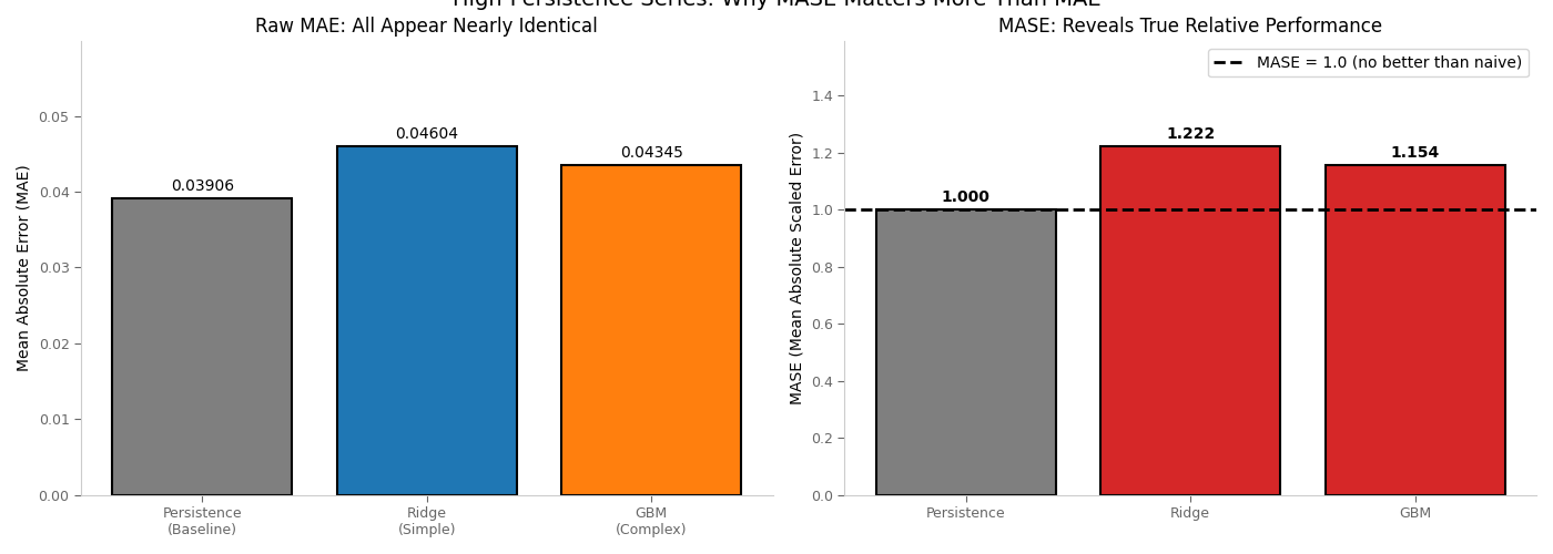
Visualization: High-Persistence Metrics Comparison

This plot shows why MASE matters for high-persistence series and compares model performance relative to the persistence baseline.

# Generate data and fit models for visualization
series = generate_high_persistence_data()
X, y = create_features(series)
train_size = int(0.7 * len(y))
X_train, X_test = X[:train_size], X[train_size:]
y_train, y_test = y[:train_size], y[train_size:]

# Fit models
ridge = Ridge(alpha=1.0)
ridge.fit(X_train, y_train)
ridge_preds = ridge.predict(X_test)

gbm = GradientBoostingRegressor(n_estimators=50, max_depth=2, random_state=42)
gbm.fit(X_train, y_train)
gbm_preds = gbm.predict(X_test)

# Persistence baseline
persistence_preds = X_test[:, 0]

# Compute metrics
persistence_mae = np.mean(np.abs(y_test - persistence_preds))
ridge_mae = np.mean(np.abs(y_test - ridge_preds))
gbm_mae = np.mean(np.abs(y_test - gbm_preds))

ridge_mase = compute_mase(y_test, ridge_preds, train_data=y_train)
gbm_mase = compute_mase(y_test, gbm_preds, train_data=y_train)

# Create visualization
fig, axes = plt.subplots(1, 2, figsize=(14, 5))

# Left: MAE comparison (shows why raw MAE is misleading)
ax1 = axes[0]
models = ["Persistence\n(Baseline)", "Ridge\n(Simple)", "GBM\n(Complex)"]
maes = [persistence_mae, ridge_mae, gbm_mae]
colors = ["#7f7f7f", "#1f77b4", "#ff7f0e"]
bars = ax1.bar(models, maes, color=colors, edgecolor="black", linewidth=1.5)
ax1.set_ylabel("Mean Absolute Error (MAE)")
ax1.set_title("Raw MAE: All Appear Nearly Identical")
ax1.set_ylim(0, max(maes) * 1.3)

for bar, mae in zip(bars, maes):
    ax1.annotate(
        f"{mae:.5f}",
        xy=(bar.get_x() + bar.get_width() / 2, bar.get_height()),
        xytext=(0, 3),
        textcoords="offset points",
        ha="center",
        va="bottom",
        fontsize=10,
    )

# Right: MASE comparison (reveals true relative performance)
ax2 = axes[1]
models_mase = ["Persistence", "Ridge", "GBM"]
mases = [1.0, ridge_mase, gbm_mase]
colors_mase = [
    "#7f7f7f",
    "#2ca02c" if ridge_mase < 1 else "#d62728",
    "#2ca02c" if gbm_mase < 1 else "#d62728",
]
bars2 = ax2.bar(models_mase, mases, color=colors_mase, edgecolor="black", linewidth=1.5)
ax2.axhline(
    1.0, color="black", linestyle="--", linewidth=2, label="MASE = 1.0 (no better than naive)"
)
ax2.set_ylabel("MASE (Mean Absolute Scaled Error)")
ax2.set_title("MASE: Reveals True Relative Performance")
ax2.set_ylim(0, max(mases) * 1.3)
ax2.legend(loc="upper right")

for bar, mase in zip(bars2, mases):
    label = f"{mase:.3f}"
    if mase < 1:
        label += " ✓"
    ax2.annotate(
        label,
        xy=(bar.get_x() + bar.get_width() / 2, bar.get_height()),
        xytext=(0, 3),
        textcoords="offset points",
        ha="center",
        va="bottom",
        fontsize=10,
        fontweight="bold",
    )

# Apply Tufte styling
for ax in axes:
    apply_tufte_style(ax)

plt.tight_layout()
plt.suptitle("High-Persistence Series: Why MASE Matters More Than MAE", y=1.02, fontsize=14)
plt.show()