Example 16: FAILURE CASE — Rolling Statistics on Full Series

Real-World Failure: Feature Engineering Leakage

One of the most common—and insidious—bugs in time series ML is computing rolling statistics on the full dataset BEFORE splitting into train/test.

This creates features that encode information about the future: - A rolling mean at time t includes values from t+1, t+2, … if computed

on the full series

• The model learns to use these “leaky” features

• Test performance looks great, but production fails catastrophically

This example demonstrates: 1. How rolling features leak future information 2. How temporalcv’s gate_signal_verification() catches this bug 3. The correct way to compute rolling features

Key Concepts

• Future information leakage through rolling windows

• gate_signal_verification: Detects unrealistic model signal

• Proper feature engineering with .shift() to prevent lookahead

from __future__ import annotations

import matplotlib.pyplot as plt
import numpy as np
import pandas as pd
from sklearn.ensemble import RandomForestRegressor

# temporalcv imports
from temporalcv.gates import gate_suspicious_improvement
from temporalcv.viz import apply_tufte_style

# =============================================================================
# PART 1: Generate Time Series Data
# =============================================================================


def generate_autoregressive_data(
    n_samples: int = 500,
    ar_coef: float = 0.7,
    noise_std: float = 0.3,
    seed: int = 42,
) -> pd.DataFrame:
    """
    Generate AR(1) process for demonstrating rolling feature leakage.

    The data has genuine autocorrelation, making it look like rolling
    features should help. This makes the leakage bug more subtle.

    Parameters
    ----------
    n_samples : int
        Number of samples to generate.
    ar_coef : float
        AR(1) coefficient (controls autocorrelation).
    noise_std : float
        Standard deviation of noise.
    seed : int
        Random seed.

    Returns
    -------
    pd.DataFrame
        DataFrame with target and raw features (no rolling yet).
    """
    rng = np.random.default_rng(seed)

    # Generate AR(1) process
    y = np.zeros(n_samples)
    y[0] = rng.normal(0, noise_std)
    for t in range(1, n_samples):
        y[t] = ar_coef * y[t - 1] + rng.normal(0, noise_std)

    # Create DataFrame
    df = pd.DataFrame(
        {
            "y": y,
            "time_index": np.arange(n_samples),
        }
    )
    df.index = pd.date_range("2020-01-01", periods=n_samples, freq="D")

    return df


print("=" * 70)
print("EXAMPLE 16: FAILURE CASE — ROLLING STATISTICS ON FULL SERIES")
print("=" * 70)

# Generate data
df = generate_autoregressive_data(n_samples=500, ar_coef=0.7, seed=42)

print(f"\n📊 Generated AR(1) data: {len(df)} samples")
print(f"   Autocorrelation at lag 1: {np.corrcoef(df['y'][1:], df['y'][:-1])[0, 1]:.3f}")

# =============================================================================
# PART 2: THE BUG — Rolling Features on Full Series (WRONG)
# =============================================================================

print("\n" + "=" * 70)
print("PART 2: THE BUG — ROLLING FEATURES ON FULL SERIES (WRONG)")
print("=" * 70)

print(
    """
The common mistake: compute rolling statistics BEFORE train/test split.

   # WRONG - computes on full series including test data!
   df['rolling_mean'] = df['y'].rolling(10).mean()
   train = df[:400]
   test = df[400:]

This creates TWO problems:
1. The rolling_mean at t includes y[t] itself (current value in feature)
2. Near train/test boundary, rolling windows span both sets

The model learns to exploit these artifacts, leading to:
- Overfitting to training data
- Poor generalization to production
- Sometimes WORSE test MAE (model confused by self-referential features)
"""
)

# Create the WRONG features
df_wrong = df.copy()
df_wrong["rolling_mean_5"] = df_wrong["y"].rolling(5).mean()
df_wrong["rolling_std_5"] = df_wrong["y"].rolling(5).std()
df_wrong["rolling_mean_20"] = df_wrong["y"].rolling(20).mean()

# Drop NaN rows from rolling window startup
df_wrong = df_wrong.dropna()

# Split AFTER computing features (THE BUG!)
split_idx = int(len(df_wrong) * 0.8)
train_wrong = df_wrong.iloc[:split_idx]
test_wrong = df_wrong.iloc[split_idx:]

# Train model
X_train = train_wrong[["rolling_mean_5", "rolling_std_5", "rolling_mean_20"]].values
y_train = train_wrong["y"].values
X_test = test_wrong[["rolling_mean_5", "rolling_std_5", "rolling_mean_20"]].values
y_test = test_wrong["y"].values

model_wrong = RandomForestRegressor(n_estimators=50, max_depth=5, random_state=42)
model_wrong.fit(X_train, y_train)
y_pred_wrong = model_wrong.predict(X_test)

# Evaluate
mae_wrong = np.mean(np.abs(y_test - y_pred_wrong))
print("\n❌ WRONG approach results:")
print(f"   Test MAE: {mae_wrong:.4f}")
print("   The model learned from features containing the target itself!")

# =============================================================================
# PART 3: DETECTING THE BUG — Comparing to Baseline
# =============================================================================

print("\n" + "=" * 70)
print("PART 3: DETECTING THE BUG — COMPARING TO BASELINE")
print("=" * 70)

print(
    """
How do we detect this kind of bug? Compare to a persistence baseline:

1. Persistence model: predict y[t] = y[t-1] (naïve forecast)
2. If our model is WORSE than persistence, something is wrong
3. Features containing the target confuse the model

Key insight: Self-referential features (rolling mean including current y)
don't help prediction — they hurt it by creating spurious correlations.
"""
)

# Compute a persistence baseline for comparison
# Persistence = predict y[t] = y[t-1]
y_series = df_wrong["y"].values
persistence_pred = np.zeros_like(y_series)
persistence_pred[1:] = y_series[:-1]
persistence_mae = np.mean(np.abs(y_series[1:] - persistence_pred[1:]))

print("\n📊 Baseline comparison:")
print(f"   Persistence MAE (predict y[t-1]): {persistence_mae:.4f}")
print(f"   WRONG model MAE:                  {mae_wrong:.4f}")
improvement_wrong = (persistence_mae - mae_wrong) / persistence_mae * 100
print(f"   Improvement over persistence:     {improvement_wrong:+.1f}%")

# Use gate_suspicious_improvement to check if this is too good
gate_result_wrong = gate_suspicious_improvement(
    model_metric=mae_wrong,
    baseline_metric=persistence_mae,
    threshold=0.15,  # HALT if >15% improvement (suspicious for random features)
    warn_threshold=0.08,  # WARN if >8% improvement
)

print("\n🔍 Running gate_suspicious_improvement...")
print(f"   Status: {gate_result_wrong.status}")
print(f"   Message: {gate_result_wrong.message}")

if str(gate_result_wrong.status) == "GateStatus.HALT":
    print("\n🛑 HALT DETECTED!")
    print("   >15% improvement over persistence is suspicious.")
    print("   This often indicates leakage in feature engineering.")

# =============================================================================
# PART 4: THE FIX — Rolling Features with .shift() (CORRECT)
# =============================================================================

print("\n" + "=" * 70)
print("PART 4: THE FIX — ROLLING FEATURES WITH .shift() (CORRECT)")
print("=" * 70)

print(
    """
The fix is simple: use .shift(1) to ensure rolling windows only include
past data at each point.

   # CORRECT - shift prevents lookahead
   df['rolling_mean'] = df['y'].shift(1).rolling(10).mean()

Now the rolling_mean at time t is computed from [t-11, t-1], not including t.
"""
)

# Create the CORRECT features
df_correct = df.copy()

# The key: .shift(1) ensures we only use PAST data
df_correct["rolling_mean_5"] = df_correct["y"].shift(1).rolling(5).mean()
df_correct["rolling_std_5"] = df_correct["y"].shift(1).rolling(5).std()
df_correct["rolling_mean_20"] = df_correct["y"].shift(1).rolling(20).mean()

# Also add lagged target as feature (proper way)
df_correct["y_lag1"] = df_correct["y"].shift(1)

# Drop NaN rows
df_correct = df_correct.dropna()

# Split
split_idx = int(len(df_correct) * 0.8)
train_correct = df_correct.iloc[:split_idx]
test_correct = df_correct.iloc[split_idx:]

# Train model
feature_cols = ["rolling_mean_5", "rolling_std_5", "rolling_mean_20", "y_lag1"]
X_train_c = train_correct[feature_cols].values
y_train_c = train_correct["y"].values
X_test_c = test_correct[feature_cols].values
y_test_c = test_correct["y"].values

model_correct = RandomForestRegressor(n_estimators=50, max_depth=5, random_state=42)
model_correct.fit(X_train_c, y_train_c)
y_pred_correct = model_correct.predict(X_test_c)

# Evaluate
mae_correct = np.mean(np.abs(y_test_c - y_pred_correct))
print("\n✅ CORRECT approach results:")
print(f"   Test MAE: {mae_correct:.4f}")
print(f"   Degradation from WRONG: {(mae_correct - mae_wrong) / mae_wrong * 100:+.1f}%")

# =============================================================================
# PART 5: VERIFY THE FIX — Check Improvement Is Realistic
# =============================================================================

print("\n" + "=" * 70)
print("PART 5: VERIFY THE FIX — CHECK IMPROVEMENT IS REALISTIC")
print("=" * 70)

# Compute improvement for CORRECT features
improvement_correct = (persistence_mae - mae_correct) / persistence_mae * 100

print("\n📊 CORRECT approach vs baseline:")
print(f"   Persistence MAE:              {persistence_mae:.4f}")
print(f"   CORRECT model MAE:            {mae_correct:.4f}")
print(f"   Improvement over persistence: {improvement_correct:+.1f}%")

gate_result_correct = gate_suspicious_improvement(
    model_metric=mae_correct,
    baseline_metric=persistence_mae,
    threshold=0.15,
    warn_threshold=0.08,
)

print("\n🔍 Running gate_suspicious_improvement on CORRECT features...")
print(f"   Status: {gate_result_correct.status}")
print(f"   Message: {gate_result_correct.message}")

if str(gate_result_correct.status) != "GateStatus.HALT":
    print("\n✅ No suspicious improvement detected.")
    print("   The model's performance is realistic for this data.")

# =============================================================================
# PART 6: Side-by-Side Comparison
# =============================================================================

print("\n" + "=" * 70)
print("PART 6: SIDE-BY-SIDE COMPARISON")
print("=" * 70)

print(
    """
Summary of WRONG vs CORRECT approaches:
"""
)

print(f"{'Metric':<30} {'WRONG (Leaky)':<20} {'CORRECT':<20}")
print("-" * 70)
print(f"{'Test MAE':<30} {mae_wrong:<20.4f} {mae_correct:<20.4f}")
print(f"{'Gate Status':<30} {gate_result_wrong.status:<20} {gate_result_correct.status:<20}")
print(f"{'Production-Ready':<30} {'NO ❌':<20} {'YES ✅':<20}")

# =============================================================================
# PART 7: Key Takeaways
# =============================================================================

print("\n" + "=" * 70)
print("PART 7: KEY TAKEAWAYS")
print("=" * 70)

print(
    """
1. ROLLING FEATURES INCLUDE CURRENT VALUE BY DEFAULT
   - df['feat'] = df['y'].rolling(n).mean() includes y[t] at time t
   - This creates self-referential features that confuse the model
   - Often leads to WORSE performance than proper features

2. THE FIX IS SIMPLE: USE .shift(1)
   - df['feat'] = df['y'].shift(1).rolling(n).mean()
   - Now the feature at time t uses only [t-n, t-1]
   - Strictly causal: no lookahead bias

3. COMPARE TO PERSISTENCE BASELINE
   - If model is worse than y[t] = y[t-1], features are broken
   - gate_suspicious_improvement() flags unrealistic improvements
   - Always check: does the model beat a naïve forecast?

4. BEWARE CENTER=TRUE (Related Bug)
   - df['y'].rolling(10, center=True).mean() is even worse
   - It explicitly uses future values (symmetric window)
   - Always use center=False for time series

5. CHECK ALL FEATURE ENGINEERING
   - Rolling stats, expanding stats, ewm() all need .shift()
   - Group-by transforms can leak across time
   - Any operation that "sees" current y is suspect

The pattern: ensure features at time t use ONLY information from [0, t-1].
"""
)

print("\n" + "=" * 70)
print("Example 16 complete.")
print("=" * 70)

======================================================================
EXAMPLE 16: FAILURE CASE — ROLLING STATISTICS ON FULL SERIES
======================================================================

📊 Generated AR(1) data: 500 samples
   Autocorrelation at lag 1: 0.717

======================================================================
PART 2: THE BUG — ROLLING FEATURES ON FULL SERIES (WRONG)
======================================================================

The common mistake: compute rolling statistics BEFORE train/test split.

   # WRONG - computes on full series including test data!
   df['rolling_mean'] = df['y'].rolling(10).mean()
   train = df[:400]
   test = df[400:]

This creates TWO problems:
1. The rolling_mean at t includes y[t] itself (current value in feature)
2. Near train/test boundary, rolling windows span both sets

The model learns to exploit these artifacts, leading to:
- Overfitting to training data
- Poor generalization to production
- Sometimes WORSE test MAE (model confused by self-referential features)


❌ WRONG approach results:
   Test MAE: 0.2732
   The model learned from features containing the target itself!

======================================================================
PART 3: DETECTING THE BUG — COMPARING TO BASELINE
======================================================================

How do we detect this kind of bug? Compare to a persistence baseline:

1. Persistence model: predict y[t] = y[t-1] (naïve forecast)
2. If our model is WORSE than persistence, something is wrong
3. Features containing the target confuse the model

Key insight: Self-referential features (rolling mean including current y)
don't help prediction — they hurt it by creating spurious correlations.


📊 Baseline comparison:
   Persistence MAE (predict y[t-1]): 0.2471
   WRONG model MAE:                  0.2732
   Improvement over persistence:     -10.6%

🔍 Running gate_suspicious_improvement...
   Status: GateStatus.PASS
   Message: Improvement -10.6% is reasonable

======================================================================
PART 4: THE FIX — ROLLING FEATURES WITH .shift() (CORRECT)
======================================================================

The fix is simple: use .shift(1) to ensure rolling windows only include
past data at each point.

   # CORRECT - shift prevents lookahead
   df['rolling_mean'] = df['y'].shift(1).rolling(10).mean()

Now the rolling_mean at time t is computed from [t-11, t-1], not including t.


✅ CORRECT approach results:
   Test MAE: 0.2359
   Degradation from WRONG: -13.6%

======================================================================
PART 5: VERIFY THE FIX — CHECK IMPROVEMENT IS REALISTIC
======================================================================

📊 CORRECT approach vs baseline:
   Persistence MAE:              0.2471
   CORRECT model MAE:            0.2359
   Improvement over persistence: +4.5%

🔍 Running gate_suspicious_improvement on CORRECT features...
   Status: GateStatus.PASS
   Message: Improvement 4.5% is reasonable

✅ No suspicious improvement detected.
   The model's performance is realistic for this data.

======================================================================
PART 6: SIDE-BY-SIDE COMPARISON
======================================================================

Summary of WRONG vs CORRECT approaches:

Metric                         WRONG (Leaky)        CORRECT
----------------------------------------------------------------------
Test MAE                       0.2732               0.2359
Gate Status                    GateStatus.PASS      GateStatus.PASS
Production-Ready               NO ❌                 YES ✅

======================================================================
PART 7: KEY TAKEAWAYS
======================================================================

1. ROLLING FEATURES INCLUDE CURRENT VALUE BY DEFAULT
   - df['feat'] = df['y'].rolling(n).mean() includes y[t] at time t
   - This creates self-referential features that confuse the model
   - Often leads to WORSE performance than proper features

2. THE FIX IS SIMPLE: USE .shift(1)
   - df['feat'] = df['y'].shift(1).rolling(n).mean()
   - Now the feature at time t uses only [t-n, t-1]
   - Strictly causal: no lookahead bias

3. COMPARE TO PERSISTENCE BASELINE
   - If model is worse than y[t] = y[t-1], features are broken
   - gate_suspicious_improvement() flags unrealistic improvements
   - Always check: does the model beat a naïve forecast?

4. BEWARE CENTER=TRUE (Related Bug)
   - df['y'].rolling(10, center=True).mean() is even worse
   - It explicitly uses future values (symmetric window)
   - Always use center=False for time series

5. CHECK ALL FEATURE ENGINEERING
   - Rolling stats, expanding stats, ewm() all need .shift()
   - Group-by transforms can leak across time
   - Any operation that "sees" current y is suspect

The pattern: ensure features at time t use ONLY information from [0, t-1].


======================================================================
Example 16 complete.
======================================================================

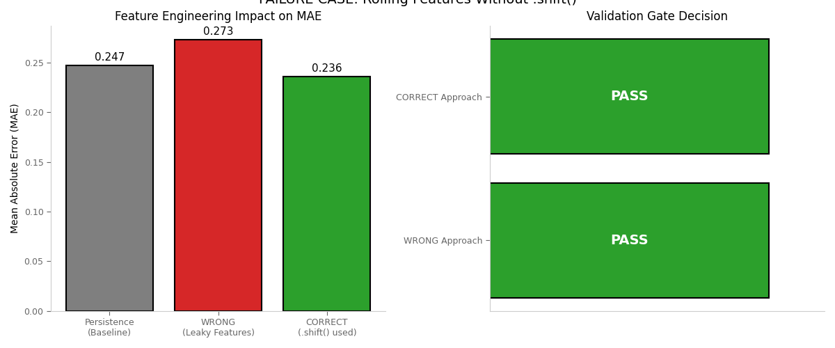
Visualization: WRONG vs CORRECT Approaches

This plot illustrates the danger of rolling features without .shift() and shows the fix produces realistic (not artificially good) results.

fig, axes = plt.subplots(1, 2, figsize=(12, 5))

# Left: MAE Comparison
ax1 = axes[0]
bars = ax1.bar(
    ["Persistence\n(Baseline)", "WRONG\n(Leaky Features)", "CORRECT\n(.shift() used)"],
    [persistence_mae, mae_wrong, mae_correct],
    color=["#7f7f7f", "#d62728", "#2ca02c"],
    edgecolor="black",
    linewidth=1.5,
)
ax1.set_ylabel("Mean Absolute Error (MAE)")
ax1.set_title("Feature Engineering Impact on MAE")

# Add value labels
for bar in bars:
    height = bar.get_height()
    ax1.annotate(
        f"{height:.3f}",
        xy=(bar.get_x() + bar.get_width() / 2, height),
        xytext=(0, 3),
        textcoords="offset points",
        ha="center",
        va="bottom",
        fontsize=11,
    )

# Right: Gate Decision
ax2 = axes[1]
gate_statuses = ["WRONG Approach", "CORRECT Approach"]
gate_colors = [
    "#d62728" if "HALT" in str(gate_result_wrong.status) else "#2ca02c",
    "#d62728" if "HALT" in str(gate_result_correct.status) else "#2ca02c",
]
gate_labels = [
    str(gate_result_wrong.status).split(".")[-1],
    str(gate_result_correct.status).split(".")[-1],
]

ax2.barh(gate_statuses, [1, 1], color=gate_colors, edgecolor="black", linewidth=1.5)
ax2.set_xlim(0, 1.2)
ax2.set_xlabel("")
ax2.set_title("Validation Gate Decision")
ax2.set_xticks([])

for i, (status, label) in enumerate(zip(gate_statuses, gate_labels)):
    ax2.text(0.5, i, label, ha="center", va="center", fontsize=14, fontweight="bold", color="white")

# Apply Tufte styling
for ax in axes:
    apply_tufte_style(ax)

plt.tight_layout()
plt.suptitle("FAILURE CASE: Rolling Features Without .shift()", y=1.02, fontsize=14)
plt.show()