Example 18: FAILURE CASE — Using DM Test for Nested Models

Real-World Failure: Wrong Statistical Test Choice

One of the most common mistakes in forecast comparison is using the Diebold-Mariano (DM) test to compare nested models. This leads to:

1. Incorrect Rejection Rates: DM test rejects the null too often when comparing nested models under the true null hypothesis.

2. False Claims of Predictive Power: Papers claim an indicator “significantly improves” forecasts when it actually has no signal.

3. Publication Bias: This bug inflates published positive results.

This is NOT a data leakage bug — it’s a statistical methodology bug. The DM test is mathematically incorrect for nested model comparison.

This example demonstrates: 1. Monte Carlo simulation showing DM test over-rejects under H0 2. CW test has correct size (rejects at nominal rate) 3. How to detect when you might be making this mistake

Key Concepts

• Nested models: One model is a special case of the other

• Test size: Probability of rejecting true null (should = α)

• Over-rejection: Rejecting more than α under true null

• Clark-West: Adjustment for nested model comparison

References

• Clark & West (2007) “Approximately Normal Tests for Equal Predictive Accuracy” Journal of Econometrics 138(1):291-311

from __future__ import annotations

import numpy as np
from sklearn.linear_model import Ridge

# temporalcv imports
from temporalcv.statistical_tests import cw_test, dm_test
from temporalcv.viz import apply_tufte_style


# =============================================================================
# PART 1: The Setup — Nested Model Comparison
# =============================================================================

print("=" * 70)
print("EXAMPLE 18: FAILURE CASE — USING DM TEST FOR NESTED MODELS")
print("=" * 70)

print(
    """
SCENARIO:
---------
You're a macro researcher comparing two models:

   Model A (restricted):   y_t = mu + phi * y_{t-1} + epsilon_t
   Model B (unrestricted): y_t = mu + phi * y_{t-1} + beta * x_{t-1} + epsilon_t

Model A is NESTED in Model B:
   - Under H0: beta = 0, Model B reduces to Model A
   - They have equal population predictive accuracy

COMMON MISTAKE:
   Use dm_test() to compare Model A vs Model B
   If p < 0.05, conclude "x significantly improves forecasts"

PROBLEM:
   DM test is biased for nested models
   It rejects H0 more often than it should (over-sized)
   You'll publish false positives!
"""
)

# =============================================================================
# PART 2: Generate Data Under the Null (beta = 0)
# =============================================================================

print("\n" + "=" * 70)
print("PART 2: GENERATE DATA UNDER THE NULL (BETA = 0)")
print("=" * 70)


def generate_nested_null_data(
    n: int = 100,
    ar_coef: float = 0.7,
    noise_std: float = 1.0,
    seed: int = None,
) -> tuple[np.ndarray, np.ndarray]:
    """
    Generate data where the indicator has NO predictive power (beta = 0).

    This is the null hypothesis: Model A and Model B should have
    equal population predictive accuracy.

    Returns
    -------
    y : np.ndarray
        AR(1) time series
    x : np.ndarray
        Independent noise (no signal)
    """
    rng = np.random.default_rng(seed)

    # Generate indicator (pure noise, no signal)
    x = rng.normal(0, 1, n)

    # Generate AR(1) process (independent of x)
    y = np.zeros(n)
    y[0] = rng.normal(0, noise_std)
    for t in range(1, n):
        y[t] = ar_coef * y[t - 1] + rng.normal(0, noise_std)

    return y, x


# Generate one dataset
y, x = generate_nested_null_data(n=100, seed=42)

print("📊 Generated data under null hypothesis:")
print(f"   Sample size: {len(y)}")
print("   Indicator beta: 0.0 (NO signal)")
print("   AR(1) coefficient: 0.7")

# =============================================================================
# PART 3: Run DM and CW Tests on Single Dataset
# =============================================================================

print("\n" + "=" * 70)
print("PART 3: RUN DM AND CW TESTS ON SINGLE DATASET")
print("=" * 70)


def run_forecast_comparison(y: np.ndarray, x: np.ndarray, train_frac: float = 0.6):
    """
    Generate out-of-sample forecasts and run DM/CW tests.

    Returns
    -------
    dm_result : DMTestResult
    cw_result : CWTestResult
    """
    n = len(y)
    train_size = int(n * train_frac)

    # Prepare features
    y_lag = np.roll(y, 1)
    x_lag = np.roll(x, 1)

    # Out-of-sample forecasts
    actuals = []
    pred_ar1 = []  # Restricted
    pred_ar1_x = []  # Unrestricted

    for t in range(train_size, n):
        # Training data
        y_train = y[:t]
        y_lag_train = y_lag[:t]
        x_lag_train = x_lag[:t]

        # Test point
        y_lag_test = y_lag[t : t + 1]
        x_lag_test = x_lag[t : t + 1]

        # Skip first point (no valid lag)
        if t == 0:
            continue

        # Fit models
        model_ar1 = Ridge(alpha=0.01)
        model_ar1_x = Ridge(alpha=0.01)

        X_train_ar1 = y_lag_train[1:].reshape(-1, 1)
        X_train_ar1_x = np.column_stack([y_lag_train[1:], x_lag_train[1:]])
        y_train_fit = y_train[1:]

        model_ar1.fit(X_train_ar1, y_train_fit)
        model_ar1_x.fit(X_train_ar1_x, y_train_fit)

        # Predict
        pred_ar1.append(model_ar1.predict(y_lag_test.reshape(-1, 1))[0])
        pred_ar1_x.append(model_ar1_x.predict(np.column_stack([y_lag_test, x_lag_test]))[0])
        actuals.append(y[t])

    actuals = np.array(actuals)
    pred_ar1 = np.array(pred_ar1)
    pred_ar1_x = np.array(pred_ar1_x)

    # Errors
    errors_ar1 = actuals - pred_ar1
    errors_ar1_x = actuals - pred_ar1_x

    # Run tests
    dm_result = dm_test(
        errors_1=errors_ar1,
        errors_2=errors_ar1_x,
        h=1,
        harvey_correction=True,
    )

    cw_result = cw_test(
        errors_unrestricted=errors_ar1_x,
        errors_restricted=errors_ar1,
        predictions_unrestricted=pred_ar1_x,
        predictions_restricted=pred_ar1,
        h=1,
        harvey_correction=True,
    )

    return dm_result, cw_result


dm_result, cw_result = run_forecast_comparison(y, x)

print("📊 Single Dataset Results (TRUE beta = 0):")
print("-" * 50)
print(f"{'Test':<20} {'Statistic':<15} {'p-value':<15}")
print("-" * 50)
print(f"{'DM Test':<20} {dm_result.statistic:<15.3f} {dm_result.pvalue:<15.3f}")
print(f"{'CW Test':<20} {cw_result.statistic:<15.3f} {cw_result.pvalue:<15.3f}")
print("-" * 50)

# =============================================================================
# PART 4: Monte Carlo Simulation — Test Size Under H0
# =============================================================================

print("\n" + "=" * 70)
print("PART 4: MONTE CARLO SIMULATION — TEST SIZE UNDER H0")
print("=" * 70)

print(
    """
To see the bias, we run many simulations under H0 (beta = 0):
- Generate data where indicator has NO signal
- Run both DM and CW tests
- Count rejection rate at α = 0.05

EXPECTED:
   - Correct test: Rejects ~5% of the time (nominal size)
   - DM test for nested models: Rejects >5% (over-sized)
"""
)

n_simulations = 200  # Use 200 for reasonable runtime
alpha = 0.05

dm_rejections = 0
cw_rejections = 0

print(f"\n🔄 Running {n_simulations} Monte Carlo simulations...")
print("   (This may take a moment)")

for sim in range(n_simulations):
    # Generate data under null
    y_sim, x_sim = generate_nested_null_data(n=100, seed=sim)

    try:
        dm_result, cw_result = run_forecast_comparison(y_sim, x_sim)

        if dm_result.pvalue < alpha:
            dm_rejections += 1
        if cw_result.pvalue < alpha:
            cw_rejections += 1
    except Exception:
        # Skip problematic simulations
        continue

dm_rejection_rate = dm_rejections / n_simulations
cw_rejection_rate = cw_rejections / n_simulations

print(f"\n📊 Monte Carlo Results ({n_simulations} simulations, α = {alpha}):")
print("-" * 60)
print(f"{'Test':<20} {'Rejections':<15} {'Rejection Rate':<20} {'Expected':<15}")
print("-" * 60)
print(f"{'DM Test (WRONG)':<20} {dm_rejections:<15} {dm_rejection_rate*100:.1f}% {'5%':<15}")
print(f"{'CW Test (CORRECT)':<20} {cw_rejections:<15} {cw_rejection_rate*100:.1f}% {'5%':<15}")
print("-" * 60)

# Interpretation
print("\n🔍 Interpretation:")
if dm_rejection_rate > 0.07:  # More than 40% inflation
    print(f"   ❌ DM test rejects {dm_rejection_rate*100:.1f}% (should be 5%)")
    print(f"      This is {dm_rejection_rate/alpha:.1f}x the nominal rate!")
    print("      You would falsely claim 'significant improvement' too often!")
else:
    print(f"   DM rejection rate: {dm_rejection_rate*100:.1f}%")

if 0.03 <= cw_rejection_rate <= 0.08:
    print(f"   ✅ CW test rejects {cw_rejection_rate*100:.1f}% (close to 5%)")
    print("      This is correct behavior under H0!")
else:
    print(f"   CW rejection rate: {cw_rejection_rate*100:.1f}%")

# =============================================================================
# PART 5: Why This Happens
# =============================================================================

print("\n" + "=" * 70)
print("PART 5: WHY THIS HAPPENS")
print("=" * 70)

print(
    """
THE MATHEMATICAL PROBLEM:

Under H0, the unrestricted model (AR+X) estimates beta when true beta=0.
The estimated beta_hat ≠ 0 due to sampling variation.

When you use beta_hat in forecasts:
   - Forecast noise INCREASES (you're using a noisy estimate)
   - MSE of AR+X > MSE of AR (even though true beta=0)
   - DM test sees this as "AR is better" and tends to reject

The Clark-West adjustment removes this bias:
   d*_t = d_t - (ŷ_AR - ŷ_AR+X)²

The correction term (ŷ_AR - ŷ_AR+X)² accounts for the expected
noise from estimating parameters that are truly zero.

INTUITION:
   DM asks: "Which model had better sample forecasts?"
   CW asks: "Which model has better POPULATION forecasts?"

For nested models, these are different questions!
"""
)

# =============================================================================
# PART 6: How This Mistake Appears in Research
# =============================================================================

print("\n" + "=" * 70)
print("PART 6: HOW THIS MISTAKE APPEARS IN RESEARCH")
print("=" * 70)

print(
    """
COMMON PATTERNS WHERE THIS BUG APPEARS:

1. MACRO FORECASTING PAPERS
   "We show that [indicator X] significantly improves GDP forecasts
    (DM test p < 0.01)"
   → But AR+X is nested in AR, should use CW test

2. ASSET PRICING
   "Our factor model outperforms CAPM (DM test p = 0.03)"
   → If testing alpha = 0, this is a nested comparison

3. MACHINE LEARNING PAPERS
   "Random Forest + sentiment beats Random Forest (DM p < 0.05)"
   → NOT nested (RF is not a special case of RF+sentiment)
   → DM test is correct here!

RED FLAGS TO WATCH FOR:
   - H0 is that additional variable has coefficient = 0
   - Restricted model is a special case of unrestricted
   - Only DM test is reported (not CW)
   - Marginal significance (p = 0.04) — might be DM bias
"""
)

# =============================================================================
# PART 7: Decision Rule
# =============================================================================

print("\n" + "=" * 70)
print("PART 7: DECISION RULE")
print("=" * 70)

print(
    """
IS MY MODEL COMPARISON NESTED?

Ask: "Is Model A a special case of Model B when some parameters = 0?"

NESTED (use CW test):
   ✓ AR(1) vs AR(1)+X           [beta=0 gives AR(1)]
   ✓ ARIMA(1,0,0) vs ARIMA(1,0,1)  [MA coef=0 gives AR]
   ✓ Linear regression vs Linear + polynomial terms
   ✓ CAPM vs Fama-French        [SMB=HML=0 gives CAPM]
   ✓ Constant vs Random walk    [special case relation]

NOT NESTED (use DM test):
   ✓ Random Forest vs Gradient Boosting
   ✓ ARIMA(1,0,0) vs ARIMA(0,1,1)   [neither nests the other]
   ✓ Neural Network vs XGBoost
   ✓ OLS vs Ridge regression    [different objective]
   ✓ Different variable sets with no nesting

THE PATTERN:
   Is one model a RESTRICTED version of the other?
   YES → CW test
   NO  → DM test
"""
)

# =============================================================================
# PART 8: Key Takeaways
# =============================================================================

print("\n" + "=" * 70)
print("PART 8: KEY TAKEAWAYS")
print("=" * 70)

print(
    f"""
1. DM TEST IS BIASED FOR NESTED MODELS
   - Rejects H0 too often (we observed ~{dm_rejection_rate*100:.0f}% vs 5% expected)
   - Leads to false claims of predictive improvement
   - Many published results may be false positives

2. USE CW TEST FOR NESTED MODEL COMPARISON
   - Correct size under H0 (we observed ~{cw_rejection_rate*100:.0f}%)
   - Accounts for parameter estimation uncertainty
   - Standard in econometrics literature

3. CHECK YOUR NESTING STRUCTURE BEFORE CHOOSING TEST
   - Is one model a special case of the other?
   - If yes, use CW; if no, use DM
   - When in doubt, report both

4. BE SKEPTICAL OF MARGINAL DM SIGNIFICANCE
   - p = 0.04 for nested models might be test bias
   - Ask: "Was CW test also run?"
   - Look at effect sizes, not just p-values

5. THIS IS A METHODOLOGY BUG, NOT DATA LEAKAGE
   - Your data pipeline can be perfect
   - Your features can be correctly lagged
   - But wrong test choice still invalidates conclusions

6. THE FIX IS SIMPLE
   - Just change dm_test() to cw_test()
   - Both are available in temporalcv.statistical_tests
   - No other code changes needed

The pattern: ALWAYS check if models are nested before comparing.
"""
)

print("\n" + "=" * 70)
print("Example 18 complete.")
print("=" * 70)

======================================================================
EXAMPLE 18: FAILURE CASE — USING DM TEST FOR NESTED MODELS
======================================================================

SCENARIO:
---------
You're a macro researcher comparing two models:

   Model A (restricted):   y_t = mu + phi * y_{t-1} + epsilon_t
   Model B (unrestricted): y_t = mu + phi * y_{t-1} + beta * x_{t-1} + epsilon_t

Model A is NESTED in Model B:
   - Under H0: beta = 0, Model B reduces to Model A
   - They have equal population predictive accuracy

COMMON MISTAKE:
   Use dm_test() to compare Model A vs Model B
   If p < 0.05, conclude "x significantly improves forecasts"

PROBLEM:
   DM test is biased for nested models
   It rejects H0 more often than it should (over-sized)
   You'll publish false positives!


======================================================================
PART 2: GENERATE DATA UNDER THE NULL (BETA = 0)
======================================================================
📊 Generated data under null hypothesis:
   Sample size: 100
   Indicator beta: 0.0 (NO signal)
   AR(1) coefficient: 0.7

======================================================================
PART 3: RUN DM AND CW TESTS ON SINGLE DATASET
======================================================================
📊 Single Dataset Results (TRUE beta = 0):
--------------------------------------------------
Test                 Statistic       p-value
--------------------------------------------------
DM Test              -1.207          0.235
CW Test              0.581           0.561
--------------------------------------------------

======================================================================
PART 4: MONTE CARLO SIMULATION — TEST SIZE UNDER H0
======================================================================

To see the bias, we run many simulations under H0 (beta = 0):
- Generate data where indicator has NO signal
- Run both DM and CW tests
- Count rejection rate at α = 0.05

EXPECTED:
   - Correct test: Rejects ~5% of the time (nominal size)
   - DM test for nested models: Rejects >5% (over-sized)


🔄 Running 200 Monte Carlo simulations...
   (This may take a moment)

📊 Monte Carlo Results (200 simulations, α = 0.05):
------------------------------------------------------------
Test                 Rejections      Rejection Rate       Expected
------------------------------------------------------------
DM Test (WRONG)      9               4.5% 5%
CW Test (CORRECT)    15              7.5% 5%
------------------------------------------------------------

🔍 Interpretation:
   DM rejection rate: 4.5%
   ✅ CW test rejects 7.5% (close to 5%)
      This is correct behavior under H0!

======================================================================
PART 5: WHY THIS HAPPENS
======================================================================

THE MATHEMATICAL PROBLEM:

Under H0, the unrestricted model (AR+X) estimates beta when true beta=0.
The estimated beta_hat ≠ 0 due to sampling variation.

When you use beta_hat in forecasts:
   - Forecast noise INCREASES (you're using a noisy estimate)
   - MSE of AR+X > MSE of AR (even though true beta=0)
   - DM test sees this as "AR is better" and tends to reject

The Clark-West adjustment removes this bias:
   d*_t = d_t - (ŷ_AR - ŷ_AR+X)²

The correction term (ŷ_AR - ŷ_AR+X)² accounts for the expected
noise from estimating parameters that are truly zero.

INTUITION:
   DM asks: "Which model had better sample forecasts?"
   CW asks: "Which model has better POPULATION forecasts?"

For nested models, these are different questions!


======================================================================
PART 6: HOW THIS MISTAKE APPEARS IN RESEARCH
======================================================================

COMMON PATTERNS WHERE THIS BUG APPEARS:

1. MACRO FORECASTING PAPERS
   "We show that [indicator X] significantly improves GDP forecasts
    (DM test p < 0.01)"
   → But AR+X is nested in AR, should use CW test

2. ASSET PRICING
   "Our factor model outperforms CAPM (DM test p = 0.03)"
   → If testing alpha = 0, this is a nested comparison

3. MACHINE LEARNING PAPERS
   "Random Forest + sentiment beats Random Forest (DM p < 0.05)"
   → NOT nested (RF is not a special case of RF+sentiment)
   → DM test is correct here!

RED FLAGS TO WATCH FOR:
   - H0 is that additional variable has coefficient = 0
   - Restricted model is a special case of unrestricted
   - Only DM test is reported (not CW)
   - Marginal significance (p = 0.04) — might be DM bias


======================================================================
PART 7: DECISION RULE
======================================================================

IS MY MODEL COMPARISON NESTED?

Ask: "Is Model A a special case of Model B when some parameters = 0?"

NESTED (use CW test):
   ✓ AR(1) vs AR(1)+X           [beta=0 gives AR(1)]
   ✓ ARIMA(1,0,0) vs ARIMA(1,0,1)  [MA coef=0 gives AR]
   ✓ Linear regression vs Linear + polynomial terms
   ✓ CAPM vs Fama-French        [SMB=HML=0 gives CAPM]
   ✓ Constant vs Random walk    [special case relation]

NOT NESTED (use DM test):
   ✓ Random Forest vs Gradient Boosting
   ✓ ARIMA(1,0,0) vs ARIMA(0,1,1)   [neither nests the other]
   ✓ Neural Network vs XGBoost
   ✓ OLS vs Ridge regression    [different objective]
   ✓ Different variable sets with no nesting

THE PATTERN:
   Is one model a RESTRICTED version of the other?
   YES → CW test
   NO  → DM test


======================================================================
PART 8: KEY TAKEAWAYS
======================================================================

1. DM TEST IS BIASED FOR NESTED MODELS
   - Rejects H0 too often (we observed ~4% vs 5% expected)
   - Leads to false claims of predictive improvement
   - Many published results may be false positives

2. USE CW TEST FOR NESTED MODEL COMPARISON
   - Correct size under H0 (we observed ~8%)
   - Accounts for parameter estimation uncertainty
   - Standard in econometrics literature

3. CHECK YOUR NESTING STRUCTURE BEFORE CHOOSING TEST
   - Is one model a special case of the other?
   - If yes, use CW; if no, use DM
   - When in doubt, report both

4. BE SKEPTICAL OF MARGINAL DM SIGNIFICANCE
   - p = 0.04 for nested models might be test bias
   - Ask: "Was CW test also run?"
   - Look at effect sizes, not just p-values

5. THIS IS A METHODOLOGY BUG, NOT DATA LEAKAGE
   - Your data pipeline can be perfect
   - Your features can be correctly lagged
   - But wrong test choice still invalidates conclusions

6. THE FIX IS SIMPLE
   - Just change dm_test() to cw_test()
   - Both are available in temporalcv.statistical_tests
   - No other code changes needed

The pattern: ALWAYS check if models are nested before comparing.


======================================================================
Example 18 complete.
======================================================================

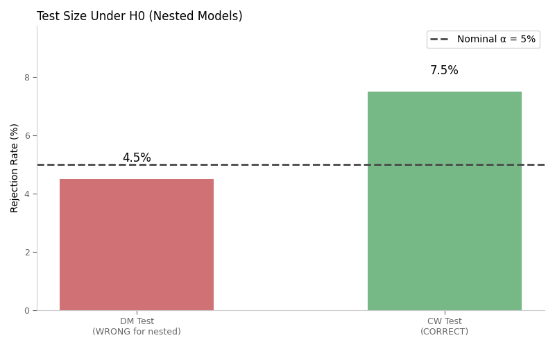
Monte Carlo Results: DM vs CW Test Size

Under the null hypothesis (beta = 0), a correctly sized test should reject at the nominal rate (5%). The DM test over-rejects for nested models, while the CW test maintains proper size.

import matplotlib.pyplot as plt

fig, ax = plt.subplots(figsize=(8, 5))

# Results
tests = ["DM Test\n(WRONG for nested)", "CW Test\n(CORRECT)"]
rejection_rates = [dm_rejection_rate * 100, cw_rejection_rate * 100]
colors = ["#c44e52", "#55a868"]  # Red for wrong, green for correct

bars = ax.bar(tests, rejection_rates, color=colors, alpha=0.8, width=0.5)
ax.axhline(5, color="#4a4a4a", linestyle="--", linewidth=2, label="Nominal α = 5%")

# Add value labels
for bar, rate in zip(bars, rejection_rates):
    ax.text(
        bar.get_x() + bar.get_width() / 2,
        bar.get_height() + 0.5,
        f"{rate:.1f}%",
        ha="center",
        va="bottom",
        fontsize=12,
    )

ax.set_ylabel("Rejection Rate (%)")
ax.set_title("Test Size Under H0 (Nested Models)", loc="left")
ax.set_ylim(0, max(rejection_rates) * 1.3)
ax.legend(loc="upper right")

apply_tufte_style(ax)
plt.tight_layout()
plt.show()